Environmental FX
Week 01: Bullet Rigid Bodies
We started this module by examining the processes and methods for using Maya's Bullet physics engine to create rigid body simulations. Rigid body simulations are employed when our simulated geometry doesn't need to be deformed. A rigid body is a polygonal or NURBS surface that has been transformed into a rigid form. Rigid bodies interact with each other during animation, unlike normal surfaces, which pass through each other.
Scene setup and scale tips
.png)
Scene setup tip: set the playhead speed to "Play every frame" to run the simulation properly.
.png)
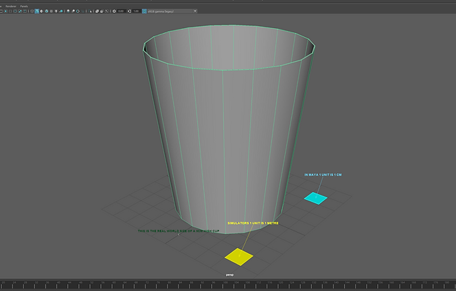
Maya internally uses 1 unit to represent 1 centimeter. However, in simulations, 1 unit is 1metre. We have to take this scale difference into account when doing simulations.
Dominos (Bullet rigid body method)
.png)
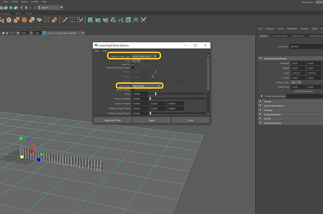
I created active rigid bodies by selecting my domino cubes and going to Bullet > Create Active Rigid Body. I set the collider shape type and body type as above.
.png)
Activated Shapes under Display menu of the outliner to be able to see and manipulate bullet rigid body shape node for each cube individually.
.png)
I made the floor a passive rigid body. Set the collider shape type and body type as above.
.png)
Under bullet rigid body shape node of the first domino cube, I manipulate the Initial Velocity value to get the first cube moving.
.png)
As explained before, in simulations, objects are in a metre unit. This leads us to have massive objects in the scene. Therefore, we need to increase the gravity value to compensate for the scaling issue.
.png)
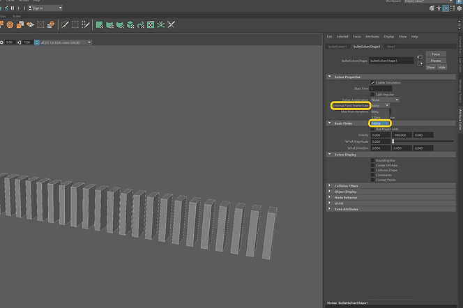
You need to change the Internal Fixed Frame Rate to 240 Hz for improved solve quality.
.png)
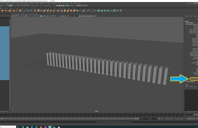
I tried to decrease the Collider Shape Margin to speed up the animation. Collider Shape Margin determines the size of the gap between Rigid objects for them to collide.
.png)
Baking a simulation allows us to generate a single animation curve for an object whose actions are being provided by simulation rather than by keys and animation curves.
Playblast (dominos falling simulation using bullet rigid bodies)
Dominos (MASH method)
.png)
I first used the pencil curve tool and drew a curve on the viewport. Then, to evenly generate and distribute control points, used Curves > Rebuild.
.png)
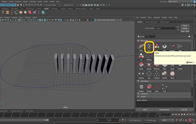
Made a Mash network and added a Curve node.
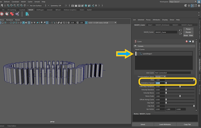.png)
Curve setup.
.png)
For the curve node to work well, we have to set Distance X to zero in Distribute options.
.png)
Increased Gravity value.
.png)
Set the Internal Frame Rate to the maximum.
.png)
Lastly, I put a domino cube there to start the domino falling. For that, I gave that domino cube a bit of rotating animation and set it as a collider (in Bullet Solver attributes). Then, as the ground seemed too slippery, I cranked up the Friction value in Bullet Solver as well as Dynamics.
Playblast (dominos falling simulation using MASH!)
Jenga Tower Play
.png)
I built a Jenga tower for this practice.
.png)
Then I chose Kinematic Rigid Body as the body type. Note: Kinematic rigid bodies can be animated during the physics simulation, but they are not affected by the simulation itself.
.png)
Headed to translateRotate node of the ball to animate it.
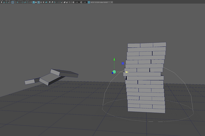.png)
Result
Playblast (Jenga with kinematic animation)
Jenga (Kinematic Dynamic animation)
.png)
Here, I wanted to animate the ball with a Kinematic rigid body, then change the body type to Dynamic when the ball is near the Jenga tower to have a nice destruction effect.
.png)
Change the body type in the channel box.
Playblast (Jenga with Kinematic Dynamic animation)
Rigid Body Shatter
.png)
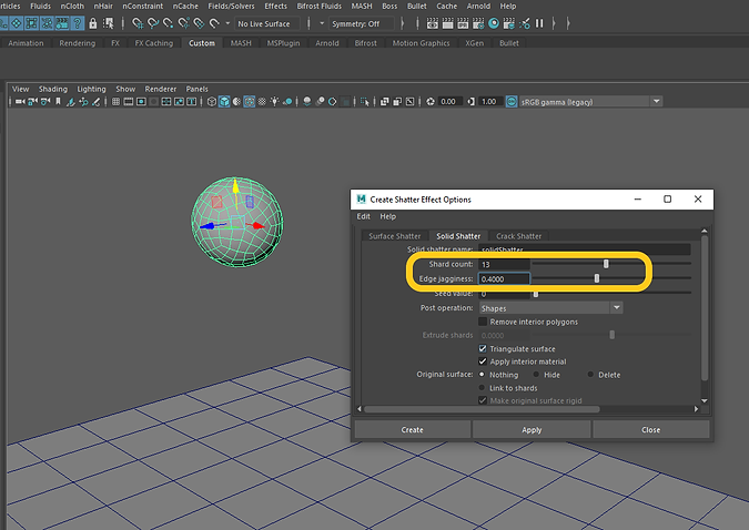
Shatter duplicates an object and breaks the duplicate into multiple pieces called shards. Note: we must first delete the objects' history ( Edit > Delete by Type > History) before creating the Shatter effect.
.png)
For the purpose of this practice, I used Solid Shatter as shown above.
.png)
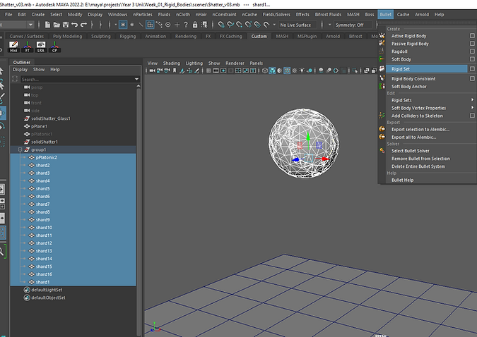
After making the shards, I grouped the ball and all the chunks to be able to position them all together in my scene.
.png)
I created a Rigid Set that comprises all the shards as well as the ball.
.png)
Changed the body type to sphere.
.png)
Made the floor a passive rigid body.
.png)
Ticked Glue Shapes and used Glue Breaking Threshold to determine how resistant the dynamic constraint is to breakage. Used a high resistance value until the ball hits the ground. The value should be set to 0 after the ball hits the floor.
.png)
As explained above, I animated the Glue Breaking Threshold value.
.png)
Set the Collision Shape Margin to 0.
.png)
I found the collision shape of the hull the best for the shattering effect.
.png)
I want the ball in my scene for the first part of the animation. Shards should be kept in the scene for the second part (after the ball hits the floor). Therefore, I exported and then imported the cache and did the trick.
.png)
Note: check the UV Write option when exporting the cache.
Render (Arnold)
Week 02: Cloth Simulation - nCloth
This week, we looked at the processes and workflows for using Maya's nCloth system to create cloth simulations. nCloth is generated from modelled polygon meshes. nCloth, Nparticles and nHair are parts of Maya's Ndynamics framework.
.png)
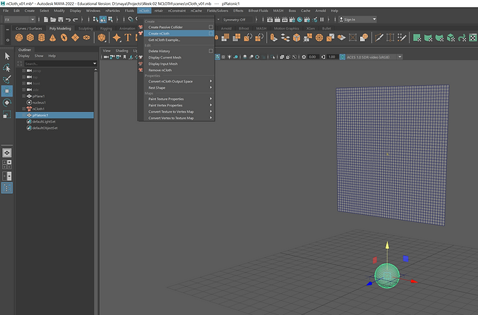
nCloth -> Create nCloth.
.png)
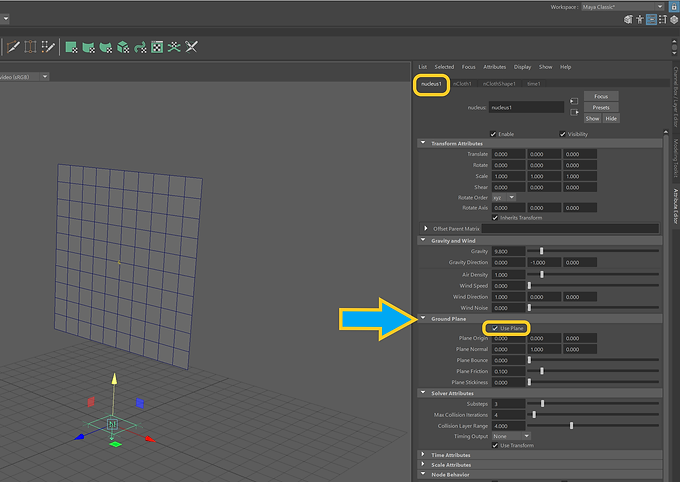
Under the nucleus node, checked "Use Plane". When on, indicates that the ground plane is used in collisions for this Maya Nucleus solver. The ground plane acts as a collision object.
.png)
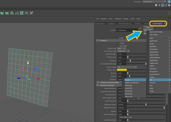
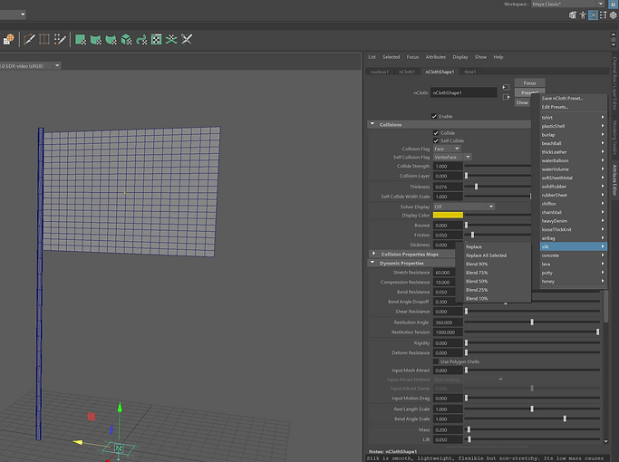
Presets section lists materials that we can create using nCloth. It provides significant attribute settings for each material.
.png)
I cranked up the number of subdivisions as having enough subdivisions is essential for the nCloth shape.
.png)
Headed to Display > Heads Up Display > Frame Rate. The frame rate appeared in the lower right-hand side of my current view.
.png)
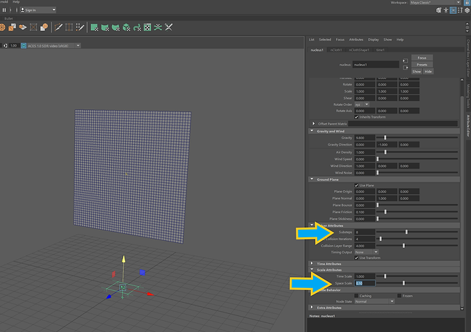
Set up substeps and space scale attributes. The Substeps attribute specifies the number of times this Maya Nucleus solver calculates per frame. Space Scale determines the relative space scale applied to this Maya Nucleus solver.
.png)
Made a ball and made it nCloth shape.
.png)
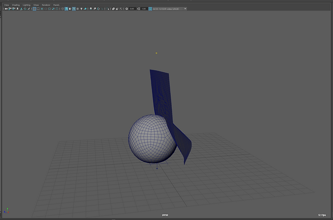
A preset selected.
.png)
Result.
Creating a waving flag using nCloth
.png)
In this practice, I wanted to make a flag waving in the wind.
.png)
Used a plane as my nCloth shape.
.png)
Ticked the "Use plane" box.
.png)
Chose a preset.
.png)
Selected a few vertices of the flag and the flag pole, then used nConstraint -> Point to Surface.
.png)
Made the flag pole a passive collider.
.png)
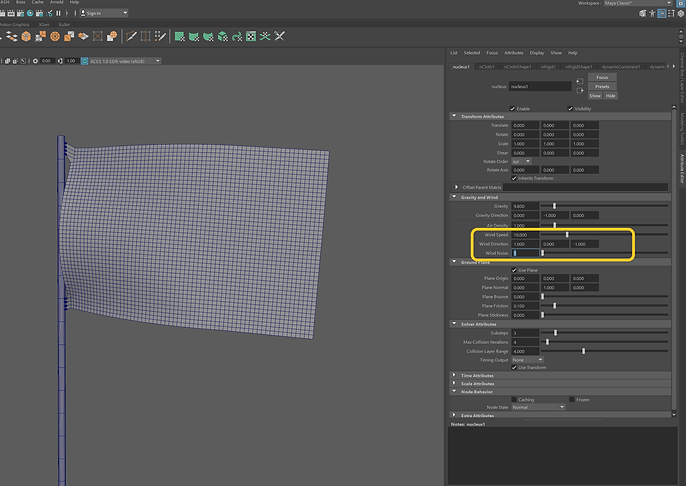
Manipulate the wind settings of the nucleus.
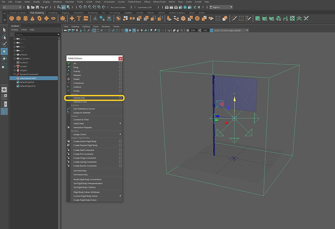.png)
Instead of using wind settings of the nucleus, here I added Volume Axis, which gave more control over the wind simulation.
.png)
The settings I used are as above.
.png)
Applied a checker board to the flag.
Waving flag (Playblast)
Making a basic skirt for a character
.png)
Here is the character I brought into my scene from Content Browser.
.png)
I then tried to make a basic skirt for the character.
.png)
Used point to surface nConstraint.
.png)
Passive collider created.
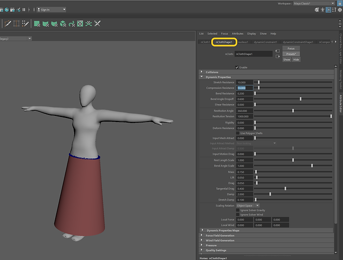.png)
Played around with nCloth shape settings.
.png)
Played around with nConstraint shape settings.
Playblast
Cloth tearing effect
1. Tearing with volume axis
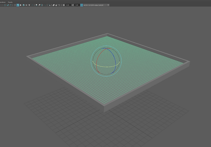.png)
I tried to simulate cloth tear in this practice.
.png)
Selected some edges and went to nConstraint -> Tearable Surface.
.png)
Volume axis created.
.png)
Chose balls as the particle type.
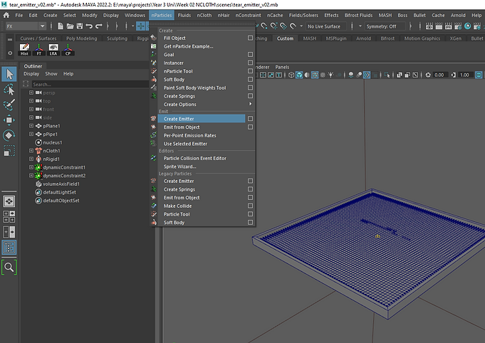.png)
Create Emitter selected.
Playblast
2. Tearing without volume axis
.png)
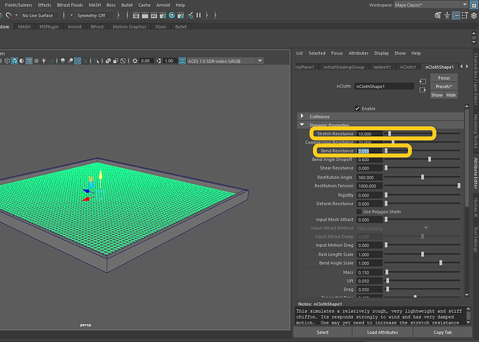
This time though, I tried to play around with nCloth and nParticle shape settings and simulate the tear without a volume axis. I changed the attributes of nCloth as above.
.png)
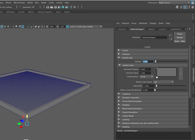
nParticle settings.
.png)
In nParticleShape settings, increased the Mass attribute.
Playblast
Week 03: Bifrost Graph Particles
This week, we learned about the Bifrost Graph and how to make particles and simulations in Maya Bifrost. We used the Bifrost Graph Editor to view, create, and alter graphs.
Note: The logic behind Bifrost Graph Editor is that we bring in an object, access some of its data, do something to its data, and then apply it to the object.
Bifrost Graph basics
Basic particles graph
Collider / Setting up colour
Inherit colour from emitter
Vary source properties (colour, speed, size)
Modifier influence / Modulate influence
Turbulence influnece/ Drag influence
Rendering colour with Arnold/ Showing colours in viewport
Week 04: Bifrost Graph Aero System
Basic aero setup / source air settings
Caching
Collider settings
Solver settings
Assigning material
Vary source property
Vorticity Influence / Modulate Influence
Turbulence influence / Render settings
Week 05: Bifrost Graph Combustion Aero System
Combustion Set up / Vary Source properties
Rebel Pack Influences
Assignment 01: Artefact Destruction and Cloth
PART 1
I was asked to make a "destruction" scene in Maya for the first part of assignment #1. Bullet Rigid Bodies were utilised for this section. My main focus was on the simulation's realism and believability, as well as its renders.
Screen recording
PART 2
For the second part of this assignment, I had to use Maya's cloth systems to show how fabric could move. As a result, I worked on a precise Maya simulation of a real-world fabric event.
Screen recording
Week 08: Bifrost Fluids
We had a look at Bifrost Fluids this week. Bifröst is a simulation system for high-quality liquid and fluid effects. I experimented with Bifrost Fluids and used some essential workflows and techniques as below.
.png)
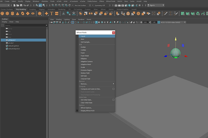
Added a platonic solid the the scene and made it a liquid emitter.
.png)
Increased the size of the liquid particles.
.png)
Made the floor a collider.
.png)
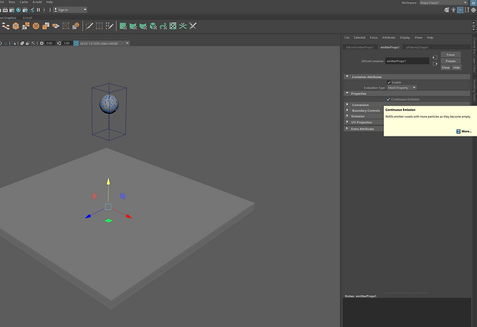
In emitter properties, selected Continuous Emission.
.png)
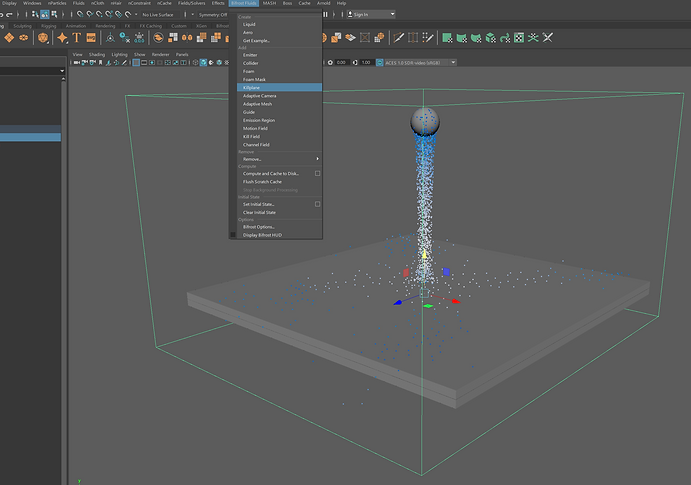
Added Killplane. This reduces the total number of particles as well as the volume that needs to be voxelized, and can reduce the memory and computational requirements.
.png)
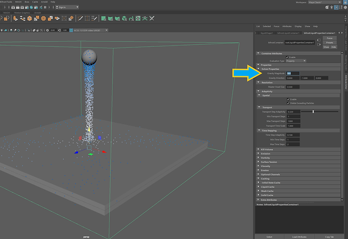
To set the scaling thing correctly, I changed the Gravity.
.png)
Density also set as above.
.png)
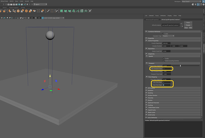
Other attributes I changed are as above.
.png)
Added another collider to the scene.
.png)
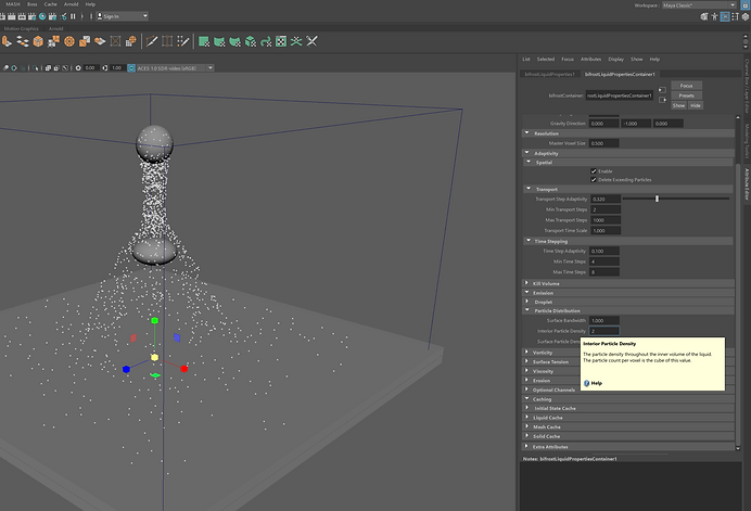
Surface Particle Density was also set. This determines the particle density at the surface of the liquid.
.png)
I also set the Interior Particle Density, which is the particle density throughout the inner volume of the liquid.
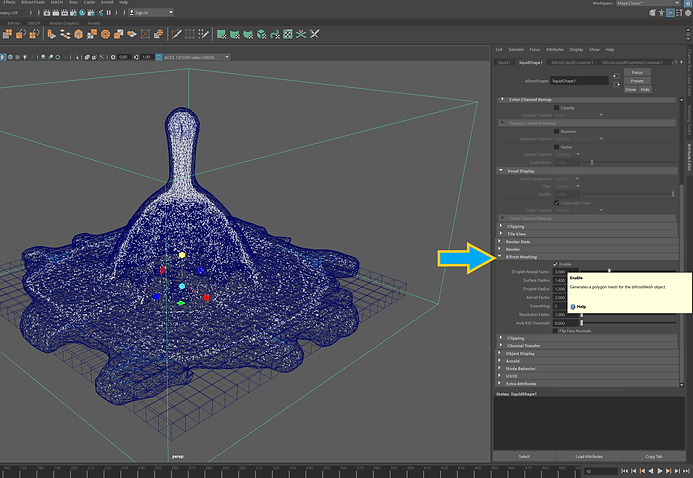.png)
Meshing enabled.
.png)
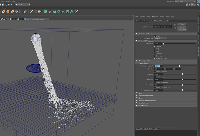
Used a Motion Field to influence the velocities of liquid.
.png)
Field direction attributes.
.png)
Here I played around with the Drag attributes.
.png)
Turbulence attributes.
.png)
The point size was reduced.
.png)
Enhanced the resolution by reducing the amount of Master Voxel Size.
.png)
Meshing enabled.
.png)
Disabled Delete Exceeding Particles.
.png)
Cached out to disk.
.png)
Caching options.
.png)
Bifrost meshing properties were set as above.
.png)
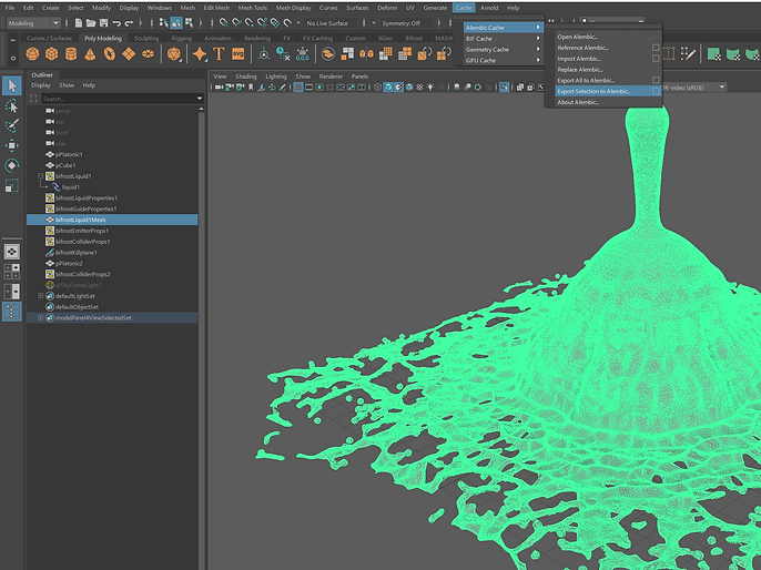
Mesh was cached out to Alembic.
.png)
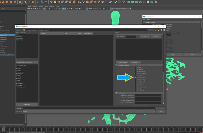
Write Color Sets should be ticked.
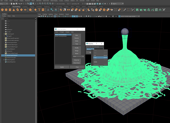.png)
The mesh colour set was copied.
.png)
I then put the colour set name to Motion Vector Source and changed the Motion Vector Unit to Per Second.
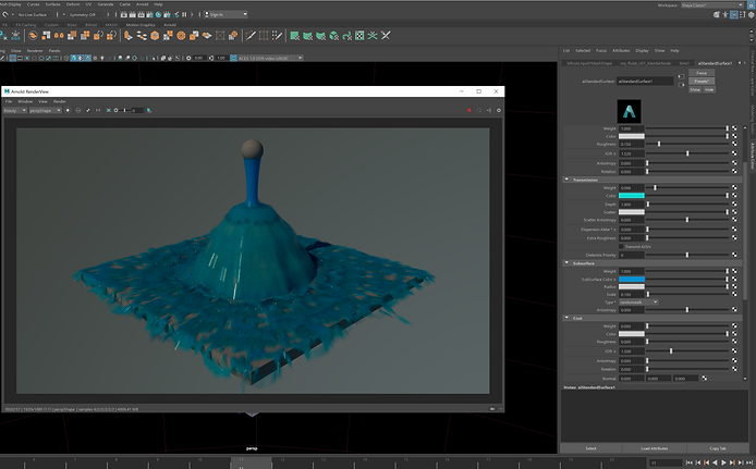.png)
aiStandardSurface attributes were manipulated to create my preferred material.
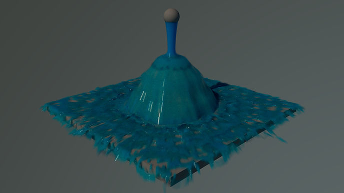
A render.
Week 09: Bifrost Ocean Simulation System - Guided Sim
We looked at Bifrost Ocean Simulation System (BOSS) this week. I experimented with guided simulation during the lecture and simulated a low-resolution ocean. Some of the most important steps are shown below:
.png)
I created a plane with the shown attributes, then headed to Boss -> Boss Editor -> Create Spectral Waves
.png)
BOSS Spectral Wave attributes set as above. For more information, click here.
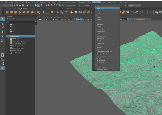.png)
To generate liquid, headed to Bifrost Liquid -> Liquid.
.png)
The surface of a Bifröst liquid simulation can be guided by a deforming plane or another flat mesh, and emission regions can be used to limit the simulation to one or more particular places. This is advantageous for images of a boat on the ocean where a big body of water must be rendered even while splashes and other simulated effects are only required for a small area of it.
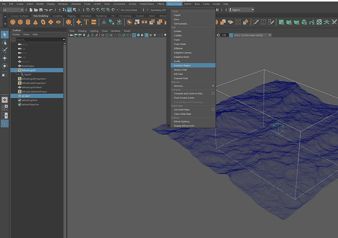.png)
Created a cube and set it as the emission region. Liquid emission volume is determined by emission regions. Memory and processing time are conserved by limiting the emission in this way.
.png)
Emission region properties are set as above.
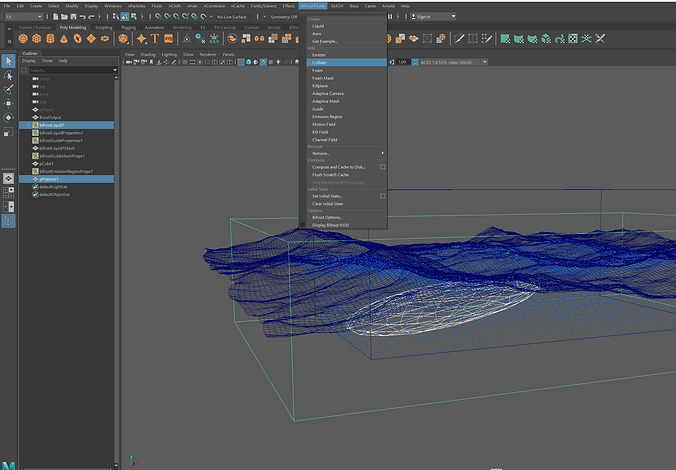.png)
I made a simple animation for a shape similar to a submarine or watercraft. I made this watercraft a collier.
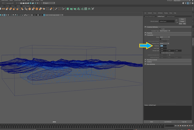.png)
Set the collier properties.
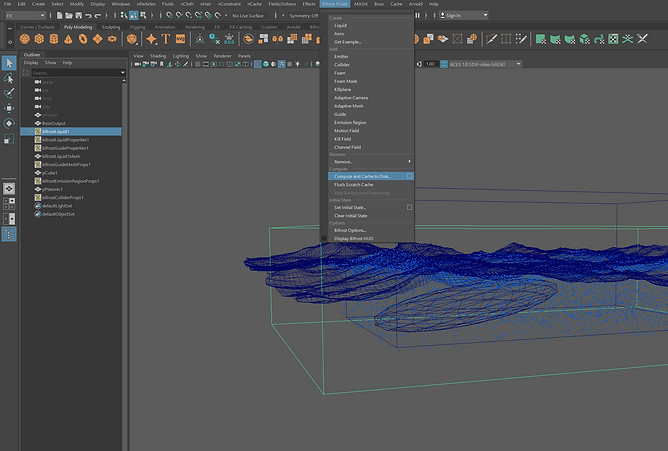.png)
Cashed the simulation to disk.
.png)
Selected the liquid in the outliner and headed to Bifrost Fluids -> Foam to add foam to the liquid.
.png)
Foam properties are set as above.
.png)
Cached out again, but this time set the write mode to Read/Write. Read/Write reads existing cache files each frame, while creating files for uncached frames based on the previously cached frames.
.png)
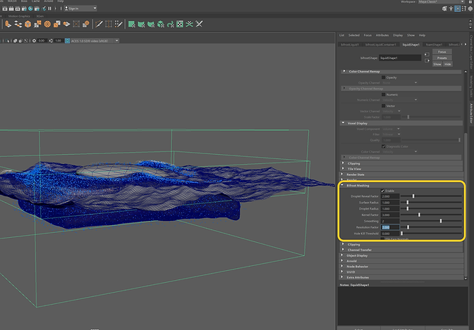
Enabled meshing with setting up above-shown attributes.
.png)
I then exported the Bifrost liquid mesh to Alembic.
.png)
My basic setup is ready, so I can now enlarge the original plane and crank up the resolution of the liquid.
.png)
To render the colours properly, I have to copy the colour set name and paste it into the Motion Vector Source field and also set Motion Vector Unit to Per Second.

Result. Note: this is a very low-resolution simulation render. I still have to play around with the resolution of the simulation for a better result. I also used a very tiny amount of emission for the water material to get a better-looking result.
Creating an ocean (Youtube videos)
Week 10: Bifrost Graph MPM
This week, we had a look at Bifrost MPM simulations. The Material Point Method (MPM) can simulate a wide range from sand and snow to cloth and fibres. The Material Point Method (MPM) was made famous by its use as a snow solver in Disney’s Frozen. One of the critical advantages of MPM is that the behaviour of simulations remains consistent as resolution increases.
An excellent in-depth masterclass which introduces MPM solver capabilities and some workflows.
Some important points
.png)
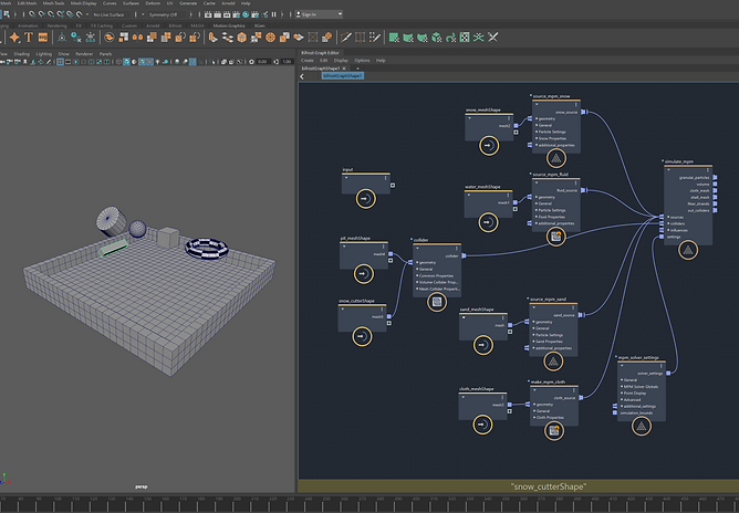
I started with a simple scene containing snow, sand, water and cloth emitters, a snow cutter and a pit collider. Then, I set up an MPM solver in Bifrost as above.
.png)
Above is the setup I used for caching out my simulations.
.png)
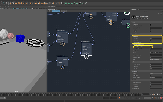
MPM solver settings. Note: Link Collider Detail
Ignores the detail size set for colliders, and uses the solver's detail size set above instead. Use this to avoid problems in cloth simulations when the detail size for colliders is very coarse compared to the detail size for cloth. If both this option and Use Mesh Resolution are on, the detail size for colliders is also computed from the input cloth mesh.
.png)
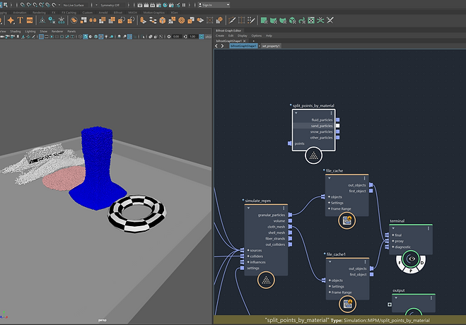
I used Split Points by Material to separate out different particles.
.png)
Above shows the setup I used for meshing the liquid.
Week 13: Bifrost Strands and Fibers
This week, we looked at strands, and learnt some useful techniques and workflows using strands in Bifrost.
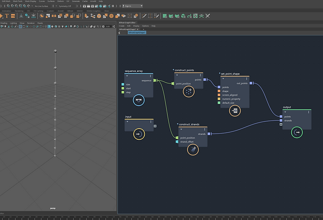.png)
I built a few points, then converted them to strands. I used set_point_shape to change the sape of points.
.png)
Set_strands_shape and set_strands_size_profile were used to alter the shape of the strands.
.png)
To break the strand into separate strands, I used a sequence_array and hooked it up to strand_offset input. Note: I had to change the value type for the sequence array to the unit, which is an unsigned integer.
.png)
Here I started fresh with a platonic solid and added the create_strands_along_normals node.
.png)
I set the shape of the strands and constructed the points.
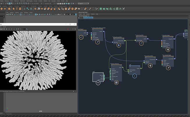.png)
I then added a fractal_turbulence node to the points as above, to add noise to the strand.
.png)
Changed the curve profile by evaluate_fcurve node.
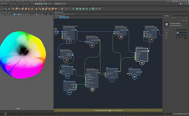.png)
Changed the curve profile by evaluate_fcurve node.
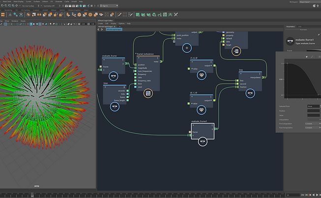.png)
Lerp node computes the linear interpolation between two values. Fraction determines the interpolation fraction. A value of 0 returns the initial value, a value of 1 returns the final value, while any other value returns the relative position on the line joining the two values.
.png)
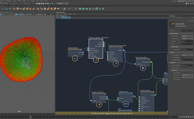
The scatter_points was used here to scatter the points across the geometry.
.png)
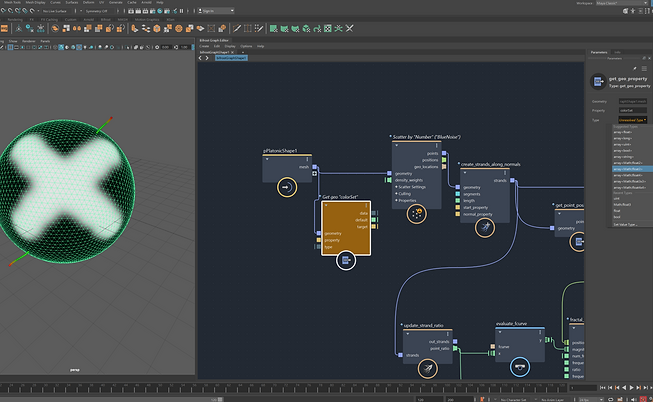
I painted vertices and then used it as the density_weights input for the scatter_points node.
.png)
Result

Render.
.png)
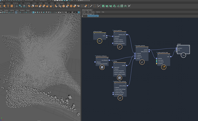
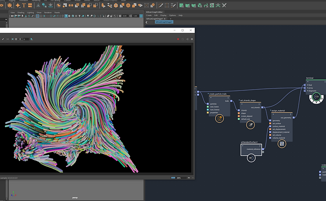
Here I wanted to play around with particle trails, so first created a basic particle system. Then used create_particle_trails node, which is part of the rebel pack.
.png)
Adding colour to the particles.
.png)
Result.

Render.
Week 12: XGEN Hair
We tried to get a grasp on XGen for hair simulation in Maya. Hair simulation is fundamentally a sculpting workflow and a career in itself. Therefore, we only looked at its basic workflows. Following are some of the results I got in the process of making hair.
.png)
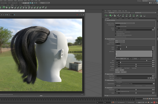
I made a basic hair set-up for a head I brought into Maya. First, I created an xGen Description. Then I sculpted guides and rebuilt them. I also added two clumping modifiers. Coil and Noise modifiers were also used to make the hair more natural.
.png)
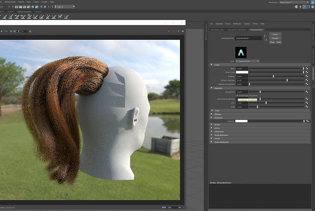
Played around with aiStandardHair shader settings.
.png)
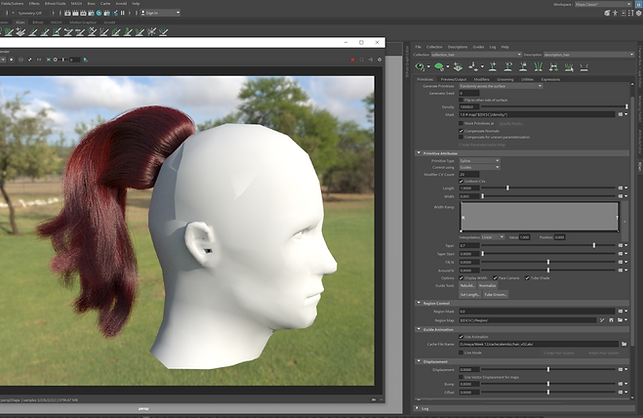
Increased hair density.
.png)
Setup Arnold render settings suitable for rendering my hair.

A render.
Week 13: Bifrost Instancing
We learnt about instancing using Bifrost this week. Instances are copies of geometric objects that are placed at point positions, such as the points of a particle system. Since only a master geometry and the points are needed for instancing, instances result in lighter scenes.
.png)
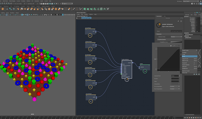
Create_instances was used to make multiple instances of the objects.
.png)
Fractal_noise_field was hooked up to the mask_weights input of the instancer to create the above effect.
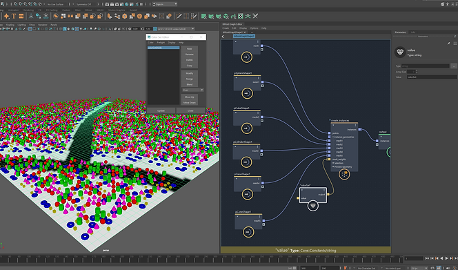.png)
I painted vertices and brought the colour set to my graph to use it as a mask.
.png)
Scatter_points was used.
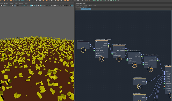.png)
I used randomise_point_... for rotation, scale and translation.
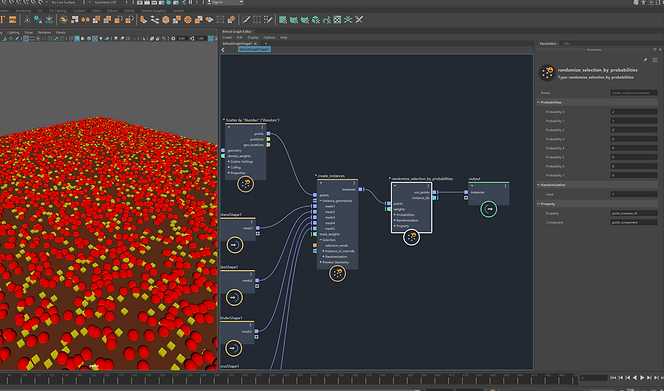.png)
I used randomise_selection_by_probabilities. It randomises the shapes placed on the points of an instances object, with control over the relative numbers of each shape.
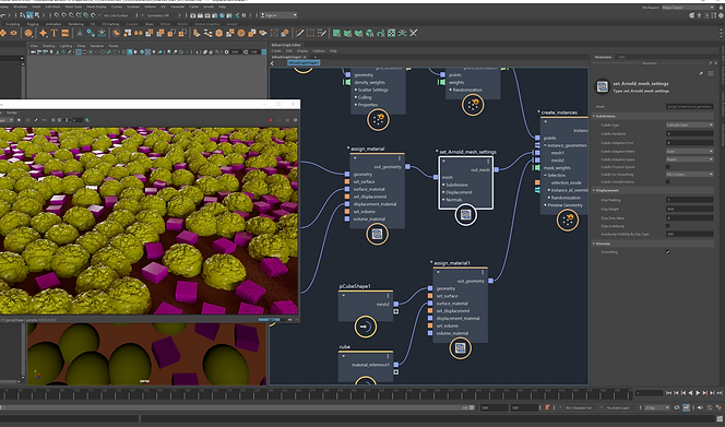.png)
Used set_Arnold_mesh_settings to give the geometry more subdivisions while rendering with Arnold for rendering displacement correctly.
.png)
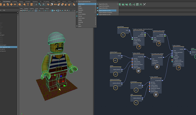
Here, I brought in a model and then exported it as a .ASS file. I could use Arnold StandIn to bring my ASS file into my scene, but instead, I would do this in Bifrost next.
.png)
ASS file was imported into bifrost by using create_archive_instances node.
.png)
A render.
Assignment 02 : Environmental Effects, Three Scenarios
Assessment task:
The assignment is to make three rendered environmental effects scenarios. These scenarios will be defined by these three titles:
Natural – Simulated environmental effect mimicking a natural phenomenon that occurs in the world.
Fantasy / Sci-Fi - Simulated environmental effect that has a fantasy or science fiction element.
Surreal - Simulated environmental effect that has an odd or unexpected element.